Sparse Image Reconstruction via L1-minimization
 |
 |
 |
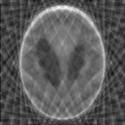
| Original | Minimum Energy Reconstruction | Sparse Reconstruction |
Introduction
This is a follow up of the L1-minimization series. The previous two posts are:
- A Comparison of Least Square, L2-regularization and L1-regularization
- Sparse Signal Reconstruction via L1-minimization
We have explored using L1-minimization technique to recover a sparse signal. The example shows a 1D example. This post demonsrates on a 2D example, where the image is viewed as a signal. This makes sense as we can perform 2D Fourier Transform in the image, where the basis are a combination of horizontal and vertical waves. For a complete introduction to FFT on images, refer to this tutorial. Notice that similar to 1D signal, we do not measure the image directly in time domain, but we do it in the frequency domain. Concretely, say \(x\) is the 2D image collapsed to 1D, and \(A \in \reals^{k\times n}\) is the measurement matrix, \(b\) is the observation, we then have \(Ax=b\). Usually we will require \(k = n\) to obtain an exact solution for \(x\) given \(A\) and \(b\). Now, if we use FFT and obtain the frequency coefficients as \(\hat{x}\), we can also perform similar measurements \(\hat{A} \hat{x} = \hat{b}\), and the requirement \(k = n\) is the same. In other words, the required samples (the information) is the same. By using the inverse fourier transform, we can convert \(\hat{x}\) back to \(x\). The only difference is that the measurement \(\hat{A}\) is taken in frequency (Fourier) domain. As we can see later, we can utilize sparse information to reduce \(k\).
Image Gradients and Total Variation
We first introduct the concept of image gradients. For any 2D real image I, if
we think about each row as a signal, we can then view the ‘difference’ between
adjacent pixels as (horizontal) gradient Gx(I), this makes sense since a
sharpe change denotes an edge. Similary, we can define the vertical gradient
Gy(I) for columns. Thus, we have
where the image size is \(n\times n\).
Collectively, the image gradient G(I) is defined as the
magnitude (2-norm) of both components:
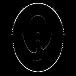
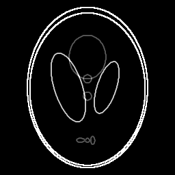
The following shows Gx, Gy and G of the phantom image:
 |
 |
 |
Gx(I) |
Gy(I) |
G(I) |
The total variation TV(I) of an image is just the sum of
this discrete gradient at every point.
We notice that \(TV(I)\) is just the L1-norm of \(G(I)\), which leads us to the following: if we have an image that is sparse in its image gradients, we can exploit that and use our L1-minimization trick.
Sparse Gradient Image Reconstruction
The ratio of non-zero elements in Gx, Gy and G of the phantom image
is 0.0711, 0.0634 and 0.0769, respectively. These ratios are really
small - and we consider the gradient as sparse.
Let \(F: \reals^{n\times n} \to \complex^{n\times n}\) be the FFT operator, and \(F I\) be the Fourier transform taken on image I. Define a set \(\Omega\) as the \(k\) two-dimensional frequencies chosen according to some sampling pattern from the \(n \times n\). We further define \(F_\Omega I: \reals^{n \times n} \to \complex^k\) as the \(k\) observation taken from the fourier transform of image I. We can then solve the following optimization problem to recover \(I\):
\[\min_I \norm{F_\Omega I - b}^2_2\]where \(F_\Omega\) can be view as the measurement matrix, \(b\) is the observation, and we want to find \(I\) such that the reconstruction cost (energy) is minimized.
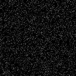
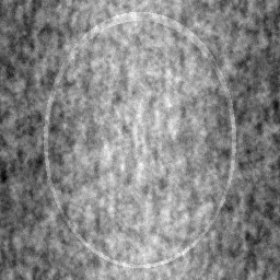
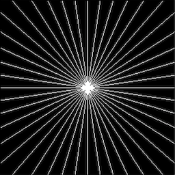
However, the above does not quite work. As we can see in the following images, the L2-minimization does a poor job, either for a random measurement or a radial measurement [@candes2006robust] in Fourier domain.
 |
 |
 |
| Random measurement | L2-minimization | L1-minimization |
 |
 |
 |
| Radial measurement | L2-minimization | L1-minimization |
To utilize the sparse information, we add a L1-regularization term to the above objective function, which yields the following:
\[(TV_1) \quad \min_I \norm{F_\Omega I - b}^2_2 + \lambda TV(I)\]Without surprise, optimizing the above gives us a perfect reconstruction of the original image. It is shown that if there exists a piecewise constant I with sufficiently few edges (i.e., \(G(I)_{ij}\) is nonzero for only a small number of indices i, j), then \((TV_1)\) will recover I exactly.
A heavily commented code example is available in my github repository. Leave a comment if you have any question.
Probing Further
Now, take a look at another example cameraman, which has the following
gradients (intensity rescaled using matlab’s imagesc.
 |
 |
| Cameraman | Gradient |
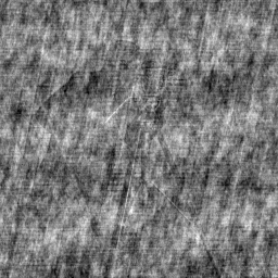
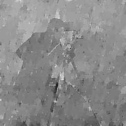
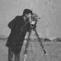
The following shows the reconstructions (left two are using random measurements, right two are using radial measurements).
 |
 |
 |
 |
| Rand (L2) | Rand (L1) | Radial (L2) | Radial (L1) |
As we can see, the results are not as good. In fact, the non-zero ratio of its gradient is 0.9928, which is not sparse at all. However, if we plot the histogram of gradients, we will find that most of the gradient magnitudes are small:
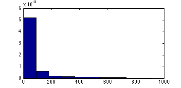
In particular, most of them are smaller than 200, which means the number of ‘changes’ that are larger than 200 is small. In fact, the ratio of gradient > 200 is only 0.0964! Thus, there are two possible ways to discard these information and get a ‘compressed’ image that is sparse in gradients:
- Use mean-shift algorithm to segment the regions such that they have the same color intensities. K-means or quantization should achieve a similar result, though might not as good as mean-shift.
- Use image filtering to smooth the image, which can effectively average colors and discard high frequency information.
I’ll leave these conjectures for furture implementation. For those intereted, please try them yourself and let me know your results. If you have any thoughts, do not hesitate to leave a comment.
References
For interested readers, the following references will be helpful. [1], [2], [3], [4]
- [1]E. Candes and J. Romberg, “l1-magic: Recovery of sparse signals via convex programming,” vol. 4, 2005.
- [2]J. S. Hesthaven, K. Chowdhary, E. Walsh, and others, “Sparse Gradient Image Reconstruction from Incomplete Fourier Measurements and Prior Edge Information,” IEEE TRANSACTIONS ON IMAGE PROCESSING, 2012.
- [3]J. K. Pant, W.-S. Lu, and A. Antoniou, “A new algorithm for compressive sensing based on total-variation norm,” in Circuits and Systems (ISCAS), 2013 IEEE International Symposium on, 2013, pp. 1352–1355.
- [4]E. J. Candès, J. Romberg, and T. Tao, “Robust uncertainty principles: Exact signal reconstruction from highly incomplete frequency information,” Information Theory, IEEE Transactions on, vol. 52, no. 2, pp. 489–509, 2006.


Comments